Everyone quotes group size, but it might be the noisiest way to measure how a rifle shoots. The mean radius vs group size debate matters because picking the right metric means fewer rounds wasted and fairer comparisons between loads. Here is how each works and when to use it.
“Group size” almost always means extreme spread: the center-to-center distance between the two shots farthest apart, usually quoted in inches or MOA. It is quick to measure with calipers, which is exactly why it became the standard. If you need the how-to, see how to measure group size in MOA.
The problem with extreme spread
Extreme spread has two weaknesses. First, it is defined entirely by your two worst shots: one flyer doubles it, and it tells you nothing about how the other shots clustered. Second, it grows with sample size: a 10-shot group will almost always measure larger than a 5-shot group from the same rifle, simply because more shots give more chances to catch an extreme pair. That makes it statistically noisy and unfair to compare across different shot counts.
What is mean radius?
Mean radius is the average distance of every shot from the group’s center (the centroid of all impacts). Because it uses all of your data instead of just the two outliers, it is far more stable and repeatable from group to group, and it barely flinches at a single flyer. In statistical terms it is a more efficient estimator: you get a trustworthy read from fewer rounds, which is precisely what a handloader testing many charges wants.
Mean radius vs group size at a glance
Metric
Uses
Strengths
Weaknesses
Extreme spread
2 widest shots
Fast, caliper-friendly, familiar
Noisy; grows with shot count; ignores the cluster
Mean radius
Every shot
Stable, efficient, fair across sample sizes
Needs software to measure each impact
CEP / R50
Every shot (probabilistic)
Robust, statistically meaningful
Less intuitive to most shooters
What about CEP and R50?
You will also see CEP (circular error probable) or R50: the radius of a circle, centered on the group, that contains 50% of your shots (with R90/R95 variants for more). It is a probabilistic cousin of mean radius and a very honest way to express precision. If you want the formal background, see circular error probable.
How many shots do you need?
Because mean radius uses every impact, it settles down with fewer rounds than extreme spread does: you can get a trustworthy read from a 5- or 10-shot group, where extreme spread would still be swinging from group to group. That efficiency is the practical reason to prefer it during load development: you reach the same confidence while burning less barrel and brass. Extreme spread, by contrast, keeps creeping upward the more you shoot, so judging a 5-shot group against a 10-shot group on extreme spread alone is comparing apples to oranges. If you only remember one thing: compare like sample sizes, and lean on mean radius when rounds are precious.
Which should you use?
For a quick caliper check or to compare against published group sizes, extreme spread is fine. For serious load comparison, deciding which charge or seating depth truly shoots better with the fewest rounds, mean radius (or CEP) wins. LoadNode reports both, in MOA and MIL, from a single photo of your target, so you never have to choose between the familiar number and the better one. Then cross-check the velocity side with a good SD.
Handloading is an adult activity. LoadNode is a logbook and analysis tool: it never provides load data. Always develop loads from current published data, start low, and work up safely.
After charge weight, seating depth is the most powerful accuracy lever you control: and the one most surrounded by jargon. This guide demystifies CBTO, jump, and jam, shows how to find where your bullet meets the rifling, how a seating-depth test is structured, and why seating depth is a pressure-sensitive variable that has to be checked against your current published load data.
COAL (cartridge overall length, sometimes OAL) is measured from the case base to the very tip of the bullet. The trouble is bullet tips, especially soft polymer or lead, vary in length, so COAL is a noisy reference. CBTO (cartridge base to ogive) is measured to a point on the bullet’s ogive using a comparator. Since the ogive is the part that actually engages the rifling, CBTO is the consistent, meaningful number for controlling how your bullet meets the lands. Use COAL to check it fits your magazine; use CBTO to tune.
Jump, jam, and touch
When a chambered bullet just contacts the rifling, it is touching the lands. Seat it deeper and the bullet has to travel a short distance: the jump: before it engages the rifling. Seat it out into the rifling and it is jammed. Jump is simply how far off the lands you seat, expressed as a CBTO difference from the touch point. Different bullets prefer different jumps: some shoot best near the lands, others are happy with plenty of jump: it is something you test, not assume.
Finding your touch point
To measure jump you first need your touch CBTO: the length at which the bullet contacts the lands in your chamber. Common methods include a dedicated tool such as a Hornady OAL gauge with a modified case, or a no-tool method using a split-neck or lightly-sized case that lets the bullet be pushed back by the lands. Either way you read the result with a bullet comparator on your calipers and record the CBTO. A reloading resource like Ultimate Reloader walks through the tooling in detail.
Running a seating-depth test
Most published test methodologies hold the charge weight constant, taken from current published load data for the exact components, and vary only seating depth.
Published seating-depth protocols differ in how they step. Most share the same shape: a wide, coarse scan to find the neighbourhood, then a repeat over a narrower range in finer increments. LoadNode does not supply increment sizes. Take them from the protocol or manufacturer guidance you are working from, and stay inside the seating range your current published load data and your magazine allow.
Shoot a group at each seating depth under consistent conditions.
Compare group size and shape across the depths, remembering that one group per depth is a very small sample: the difference between neighbouring depths is often inside the spread you would get by shooting the same load twice. Treat any apparent standout as a hypothesis, not a result.
Repeat the whole test on a different day before you read anything into it: a difference that does not reappear was most likely noise rather than a real effect of seating depth.
Change only seating depth during the test: if you move the charge too, you will not know which helped.
Pressure and safety
Seating closer to or into the lands raises pressure, sometimes sharply. Never pair a maximum charge with a jam into the lands. Because moving toward the lands changes pressure, treat any seating change in that direction as a reason to go back to current published data for your exact components rather than assuming a charge that was safe with more jump is still safe. Remember too that magazine length caps how far out you can seat if you feed from the magazine. As always, start from current published data and work up carefully.
Track CBTO and jump in LoadNode
LoadNode stores your measured jam (touch) CBTO, the jump you choose, and computes the resulting loaded CBTO for each load job: so your seating-depth experiments are recorded, not guessed at from memory. It also tracks throat erosion over the barrel’s life, which matters because your touch point moves forward as the throat wears, so last season’s jump is not this season’s. Pair it with measuring each group in MOA to judge the results objectively.
Handloading is an adult activity. LoadNode is a logbook and analysis tool: it never provides load data. Always develop loads from current published data, start low, and work up safely.
A target is a feedback sheet, and learning how to read a target, whether your shots string vertically, horizontally, or scatter round, points you toward whether your ammunition or your technique deserves the next hard look. This guide walks through what each pattern usually means and how to chase down the cause.
Before you diagnose anything, shoot enough to have a real pattern. A three-shot “string” is usually just noise: random dispersion can look like a neat line by chance. Five rounds is a sensible minimum, and ten tells you far more. Reading patterns into tiny groups is the fastest way to fix a problem you do not have.
Vertical stringing (shots up and down)
Vertical is the long-range shooter’s enemy, and at distance it is most often a velocity problem: inconsistent muzzle velocity (high SD/ES) makes some rounds land high and some low. If your vertical grows with distance, look hard at your velocity spread first: see what is a good SD for reloading and what the evidence on velocity nodes actually shows. Closer in, vertical is more often technique: inconsistent shoulder or bipod pressure, breathing, natural point of aim, or follow-through.
Horizontal stringing (shots left and right)
Horizontal dispersion outdoors is usually wind first and foremost: switching conditions push rounds laterally between shots. After wind, the usual suspects are shooter-induced: trigger control (jerking or pushing), rifle cant, parallax, and inconsistent grip or cheek pressure. If your verticals are tight but you are spraying left and right, look hard at the wind and your trigger press before blaming the load.
Round groups (no pattern)
A round, patternless group is simply the combined precision of rifle, load, and shooter on the day: the random scatter with no single dominant cause. Shrinking it means improving everything a little: more consistent ammo (lower SD, sorted brass), solid fundamentals, and ammunition your rifle shoots consistently. A round group is good news in one sense: nothing is obviously broken.
Don’t over-read a single flyer
A single shot well outside the group is a flyer, and how you treat it matters. If you called it, you felt the shot break badly from a flinch, a wobble, or a gust, it is fair to set it aside and note why. If it was unexplained, you cannot just delete it: it is real data about your load or rifle. The discipline is honesty. Marking an obvious called flyer is reasonable; throwing out every shot that hurts your group is lying to yourself. Over a larger sample, genuine flyers show up as a consistent rate, not a one-off you can wish away: another reason to shoot more rounds before drawing conclusions.
Telling load from technique apart
The fastest way to separate the two is to remove yourself from the equation. Shoot off a solid rest or bags in calm conditions. If vertical or scatter persists with a rock-steady setup and no wind, the load is the likely culprit. If the group tightens dramatically off bags, you were most likely the variable, and no amount of load tuning fixes trigger control. For more on precision fundamentals, the folks at 65 Guys are a good resource.
Read it precisely with LoadNode
Eyeballing “that looks a little vertical” only goes so far. In LoadNode you tag each hole on your target photo and it does the maths: size in MOA and MIL, mean radius, and point-of-impact offset, tied to the load and the velocity data behind it, so you can see whether that vertical lines up with a high SD. The photo itself stays on your phone. Read the target with numbers, not hunches. Browse more reloading resources to go deeper.
Handloading is an adult activity. LoadNode is a logbook and analysis tool: it never provides load data. Always develop loads from current published data, start low, and work up safely.
If you chase precision, you have heard the advice: get your SD down. But what is a good SD for reloading, what does it actually measure, and when does it even matter? This guide explains standard deviation and extreme spread in plain terms, the velocity numbers worth aiming for, why sample size changes everything, and what tends to move it.
Standard deviation (SD) of muzzle velocity describes how tightly your shots cluster around their average speed. A low SD means every round leaves the muzzle at nearly the same velocity; a high SD means they vary. It is reported in feet per second (fps) and is computed from the velocities you record over a chronograph. The math is the same standard deviation used everywhere in statistics: it just happens to be measuring velocity here.
SD vs extreme spread (ES)
Extreme spread (ES) is simpler: the highest velocity minus the lowest in your string. It is easy to understand, but it only ever reflects your two most extreme shots, so it is jumpy and, importantly, it tends to grow as you shoot more rounds (more shots mean more chances to catch an outlier). SD uses every shot and is far more stable from string to string, which is why it is the better number to compare loads by. Watch both, but lean on SD, and only once you have enough shots behind it to mean anything.
What is a good SD for reloading?
There is no universal pass/fail line, but these are the rules of thumb most precision shooters use:
SD (fps)
Interpretation
Under 10
Excellent: match-grade consistency
10–15
Good: solid for most precision shooting
15–20
Acceptable up close; marginal at long range
Over 20
High: a spread this wide is large enough to show as vertical at distance.
Treat these as guidance, not law. What actually matters is the vertical your velocity spread produces at the distance you shoot: which is the next point.
Why SD matters more at distance
At 100 yards, even a sloppy SD barely shows on paper: the bullets have not had time to separate. As distance grows, velocity differences turn into vertical differences: a faster round lands higher, a slower one lower. By the time you are stretching out past 600–1000 yards, a handful of fps of spread can mean several inches (or more) of vertical. That is why benchrest shooters at 100 yards obsess over group shape while long-range shooters obsess over SD. Run your own numbers through a ballistic calculator to estimate how that spread maps to vertical at your distance.
The sample-size trap
Here is the part that trips everyone up: an SD from three shots is almost meaningless. With so few rounds, the number bounces around wildly: you can get a single-digit SD on one three-shot string and 20+ on the next from the same load. You need roughly 10 or more shots before an SD is worth trusting, and more is better. If you are making load decisions on tiny samples, you are mostly measuring luck.
What tends to move SD
None of the following is load data. These are the process variables that most often show up as velocity spread in a chronograph string; every charge weight, powder, primer and seating decision must still come from current published manufacturer data.
Weigh every charge precisely rather than throwing by volume.
Make neck tension consistent: uniform brass prep, and annealing to keep it stable over reloads.
Brass condition shows up in the numbers: variation in case capacity and primer-pocket fit adds variables to the string, which is why sorted, uniform brass usually produces tighter velocity data than mixed-headstamp brass.
Do not read too much into one string: a single small group cannot statistically separate two charges, and the difference you think you see is usually inside the noise. See why velocity ‘nodes’ are so hard to confirm for how much shooting statistical separation actually takes.
Log temperature with every string: powders differ in how much muzzle velocity shifts with ambient temperature, so a string shot on a cold morning and one shot in summer heat may not be comparable data. Record the temperature so you can see whether that is what your numbers are showing, and check the manufacturer’s current published data for the temperature behaviour of the powder you already load.
Track it automatically
LoadNode computes live SD and ES for every charge as you enter or sync velocities from your Garmin Xero, the chronograph-correct way and with flyer awareness. Pair it with mean radius and a look at how your groups string (see how to read a target) and you have the full picture: velocity consistency and what it does on paper. LoadNode shows you the numbers; you decide.
Handloading is an adult activity. LoadNode is a logbook and analysis tool: it never provides load data. Always develop loads from current published data, start low, and work up safely.
Ask ten precision handloaders how to work up a load and you will start an argument about ladder test vs OCW. Both are established load-development procedures, both have decades of range time behind them, and both are usually presented as a way to reach a conclusion in a single afternoon. This guide keeps the comparison, because the differences between them are real and worth knowing, and then adds the part the comparison usually leaves out: a ladder test and an OCW test are data-collection procedures, not shortcuts. What either one can honestly tell you depends almost entirely on how many shots sit behind the readout.
The ladder test, usually credited to Creighton Audette, is a velocity-and-vertical method. You load single rounds at steadily increasing charge weights, taken from current published data for your exact cartridge, bullet and powder and never past the published maximum, then fire them in order at a target far enough out, often 300 yards or more, for vertical differences to become visible. Ideally you shoot the string over a chronograph. Afterwards you look for consecutive charges that land at a similar elevation and, with a chrono, a stretch where velocity barely moves from one step to the next. The full procedure, and the arithmetic behind reading it, is in our guide on how to find a velocity node.
What OCW claims
OCW, Optimal Charge Weight, was developed by Dan Newberry as a point-of-impact method. Instead of single shots up a scale, you fire round-robin groups across several charges: one shot at each charge’s target in rotation, repeated, so that wind, mirage and shooter drift are spread evenly across every charge rather than landing on whichever one you happened to shoot last. The claim is that you will find three or more consecutive charges that print to the same point of impact, a “scatter node” where the rifle stops reacting to small changes in charge, and that the middle of that window is a tolerant place to sit. OCW needs no chronograph: it reads paper, not velocity. A useful overview of round-robin ladder and group methods is worth reading alongside this.
Ladder test vs OCW: the differences that are real
Ladder test
OCW
What it reads
Velocity and vertical POI per charge
Group point-of-impact across charges
Chronograph
Strongly recommended
Optional
Rounds typically fired
Fewer (1–3 per charge)
More (round-robin groups)
Typical distance
300+ yards (for vertical)
100 yards
Firing order
Sequential, bottom to top
Rotated across charges
Conditions control
Weak: drift lands on later charges
Strong: drift shared evenly
Those differences are genuine and they should shape how you plan a range trip. What follows is what the two methods have in common, and it matters more than anything in the table.
The sample-size problem both share
A group centre is not a property of a load. It is an estimate built from a few shots, and every estimate carries its own scatter. Write your rifle’s true one-axis dispersion as sigma. The centre of an n-shot group has a standard error of sigma divided by the square root of n, so two groups fired from the identical load, with nothing whatsoever changed between them, will show centres that sit on average 1.25 × sigma × the square root of (2/n) apart.
Shots per charge
Average apparent POI shift with no real difference
1 (classic ladder step)
1.77 × sigma
2
1.25 × sigma
3 (typical OCW group)
1.02 × sigma
5
0.79 × sigma
10
0.56 × sigma
Put real units on that. A rifle averaging about 1 MOA for five shots has a per-axis sigma near 0.33 MOA. A one-shot-per-charge ladder therefore separates two identical loads by roughly 0.58 MOA on average, close to 2 inches at 300 yards, by chance alone. A three-shot OCW block separates them by about 0.34 MOA, roughly a third of an inch at 100 yards. Those are precisely the sizes both methods ask you to read as signal: the ladder as a vertical cluster, OCW as consecutive charges holding the same point of impact. The pattern you are looking at is the right size to be nothing.
What round-robin firing fixes, and what it does not
Round-robin is a genuinely good idea and OCW deserves the credit for popularising it. Rotating one shot per charge means a wind shift, building mirage, a warming barrel or a tiring shooter gets shared across every charge instead of being dumped on the ones you fired last. That removes a systematic bias, and a straight ladder fired bottom to top does not have that protection: in a sequential ladder, conditions drift and charge weight increase together, so the two are confounded by design.
What round-robin cannot do is create shots. Three rounds is three rounds however you sequence them, and every number in the table above is driven by n, not by firing order. Round-robin makes a small sample less biased. It does not make a small sample large. Those are different problems, and only one of them has been solved.
The velocity readout is no safer
Shooters who run a ladder test over a chronograph often assume the velocity side escapes all this, because velocity feels like a hard measurement. The measurement is hard. The summary statistic is not. Standard deviation estimated from a short string is one of the jumpiest numbers in reloading. If a load’s true SD is 12 fps, this is the range a single string will report 95% of the time:
Shots in the string
Reported SD from a load whose true SD is 12 fps
3
2 to 23 fps
5
4 to 20 fps
10
7 to 17 fps
20
8 to 16 fps
A three-shot string from that load can honestly report 4 fps or 21 fps, and neither reading is unusual. So when two charges in a ladder come back at 6 and 18 fps, you have not learned which load is more consistent: you have mostly learned that you fired three shots. Ten rounds is where the number starts behaving. For what those figures mean once they settle down, see what is a good SD for reloading.
Neither method is a cheat code
The honest verdict on ladder test vs OCW is that the question is smaller than it looks. Neither method is a trick for extracting a reliable answer from a handful of rounds, because no method can do that. Both are simply procedures for collecting data, and both hand you a readout whose meaning is set by sample size. Catching a genuine point-of-impact shift the size of your rifle’s own dispersion, at 95% confidence, takes something on the order of 30 rounds at each charge; five rounds at each charge catches it about a quarter of the time. The full derivation is in how to find a velocity node.
That does not make either method worthless. A ladder covers a lot of ground cheaply and gives you velocity data you can keep. OCW spends more rounds on fewer charges and controls conditions better. Both are reasonable ways to narrow a field before you spend real barrel life on the survivors. What neither can do, at the round counts they are normally run at, is crown a winner. Treat the result as a hypothesis and the method has earned its place; treat it as a verdict and you are reading noise with confidence.
How to log either method honestly
Record every shot. Including the embarrassing ones. A log that quietly loses the shots you did not like is not a smaller sample, it is a biased one, and bias does not shrink when you add rounds.
Mark called flyers, never delete them. If you called the shot as you broke it, flag it as excluded and keep it visible with the reason attached. Exclusions decided after seeing where the shot landed are how a load gets promoted on evidence that was never there.
Pool your sessions. Five separate three-shot groups at one charge say far more together than any one of them says alone. Compare pooled charges, not one group against another group.
Judge with uncertainty. A single five-shot group reading “0.6 MOA” really means something closer to “between 0.4 and 1.0 MOA.” If two charges’ intervals overlap, they are not separated. See how to measure group size in MOA.
Log the conditions. Temperature, date and string order. A result found on a cold morning and not rechecked in the afternoon has been tested once.
Change one variable at a time, so the data can attribute a change to something.
Expect “indistinguishable.” With honest round counts it is the most common correct answer, and reporting it is a result, not a failure. Two charges you cannot separate are also two charges where the choice costs you little.
How LoadNode supports both
LoadNode records either method without taking a side. A ladder logs as a charge-ladder session with every velocity captured, synced automatically from a Garmin Xero or typed in, with live SD and ES per charge. An OCW block logs the same way: each charge’s group measured straight from a photo for true MOA, mean radius and point-of-impact offset. Called flyers are flagged and excluded transparently rather than deleted, so what you excluded and why stays in the record.
What it deliberately will not do is point at a flat spot and call it a node. It used to. The arithmetic above is why it stopped. Instead it pools every group you have fired at each charge, reports dispersion as a range rather than a single confident number, says plainly when two charges are too close to call, and estimates how many more rounds at each charge it would take to separate them. Every number links back to the exact load that produced it. LoadNode never marks a charge as best, never names a node, and never tells you what to load. Browse more reloading resources to go deeper.
Handloading is an adult activity. LoadNode is a logbook and analysis tool: it never provides load data. Always develop loads from current published data, start low, and work up safely.
Spend a season around precision handloaders and sooner or later someone tells you to go out and find the node. The advice always arrives with total confidence, and it almost never arrives with a sample size. This guide covers how to find a velocity node the way the method is normally taught, and then does the part most guides skip: it works out whether a ladder of three to five rounds per step is even capable, mathematically, of telling a real velocity node apart from an ordinary run of luck. The short answer is that it is not, and the arithmetic is not close.
A velocity node is described as a span of charge weights over which muzzle velocity barely changes as you add powder: a flat spot, or plateau, in the velocity-versus-charge curve. Instead of every increment adding a predictable chunk of speed, inside the plateau a few increments hardly move the chronograph at all. The idea traces back to Creighton Audette’s ladder work and Dan Newberry’s OCW method, and the promise is genuinely appealing: sit in the middle of a plateau and velocity becomes insensitive to the small charge variations and temperature swings every handloader lives with, which should mean tighter extreme spread and steadier elevation at distance.
Nothing about that mechanism is absurd. Barrels do vibrate, pressure curves are not perfectly linear, and it is entirely plausible that some regions of the curve are flatter than others. The question this article asks is narrower and much more answerable: can the test people actually run detect such a region? That is a statistics question rather than a ballistics question, and statistics gives a clear answer.
The ladder test, as it is normally taught
The standard recipe for how to find a velocity node is the ladder test:
Take your start and maximum charges from current published load data for your exact cartridge, bullet, primer, and powder. Never exceed the published maximum.
Build a ladder of evenly spaced steps from near the start charge toward maximum, with one to five rounds on each rung.
Chronograph every shot and record every velocity, not just the averages.
Plot velocity against charge weight.
Look for consecutive rungs where the line flattens out.
Here is what a ladder looks like when it appears to work. The numbers below are illustrative only and are not a recommendation of anything. Watch the change column: it shrinks across rungs 4 to 6, then jumps again.
Rung
Velocity (fps)
Change
1
2,690
–
2
2,712
+22
3
2,731
+19
4
2,742
+11
5
2,745
+3
6
2,748
+3
7
2,761
+13
8
2,779
+18
Rungs 4 to 6 read as a flat spot and rung 5 reads as the candidate. That is exactly what the method promises you will see. It is also exactly what these eight numbers look like when nothing whatsoever is happening, which is the whole problem.
Why a short ladder cannot confirm a velocity node
A rung’s average velocity is not a property of the load. It is an estimate of a property, built from a handful of shots, and like every estimate it carries its own scatter. The uncertainty on an average is the string’s standard deviation divided by the square root of the number of shots, widened by the small-sample correction that a three-shot or five-shot string demands.
Put real numbers on it. Take a string SD of 15 fps, which is unremarkable for a decent handload. Three shots put the true average for that rung somewhere inside roughly plus or minus 37 fps at 95% confidence. Five shots narrow that to about plus or minus 19 fps. Ten shots get you to about plus or minus 11 fps. Comparing two rungs is worse than measuring one, because both estimates wobble at once: two three-shot rungs cannot resolve a genuine difference smaller than about 34 fps, and two five-shot rungs cannot resolve one smaller than about 22 fps.
Now look back at the table. That flat spot was built out of differences of 3 fps. The measurement is not capable of resolving 3 fps, or 13 fps, or in most short ladders anything below roughly 20 fps. The flat spot is not information about the powder charge. It is information about the sample size. Load identical ammunition on every rung, shoot the ladder, and flat spots will still appear, in random places, run after run, because the sampling noise is precisely the size of the effect being read. There is a well-known argument that rifle nodes are largely an illusion, and this is the arithmetic that gives it teeth.
The SD of an SD
Velocity spread is the other half of a ladder, and it is shakier still. An SD calculated from a short string is itself an estimate with a wide error bar, and almost nobody quotes it that way. At 95% confidence, the true spread behind your measured SD sits inside these multiples of the number you wrote down:
Shots in the string
True SD is somewhere between
3
0.52–6.3 × measured
5
0.60–2.9 × measured
10
0.69–1.8 × measured
20
0.76–1.5 × measured
30
0.80–1.3 × measured
Read the five-shot row slowly. A five-shot string that prints an SD of 10 fps honestly means “somewhere between 6 and 29 fps.” Two rungs printing 10 fps and 18 fps off five shots each are not distinguishable in any meaningful sense: their ranges overlap across most of their length. Ranking a ladder by five-shot SD is ranking noise, confidently. For what the number means once you have enough of them, see what is a good SD for reloading.
What it would actually take
If a real difference between two charges does exist, how much shooting proves it? Expressed in multiples of your own string SD, and asking only for an 80% chance of detecting a difference that is genuinely there:
True difference between two rungs
Rounds needed at each rung
1.0 × your SD
about 16
0.75 × your SD
about 28
0.5 × your SD
about 63
0.25 × your SD
about 250
With that same 15 fps SD, catching a genuine 15 fps gap between two rungs takes roughly 16 rounds on each of them. A genuine 8 fps gap takes about 63 on each. A ten-rung ladder at three rounds per rung spends 30 rounds and resolves none of it. Separating spread rather than average is harder again: showing that one charge’s SD is truly 20% lower than another’s needs on the order of 160 rounds at each, a third lower needs about 50 at each, and only something close to a halving is catchable inside a normal session, at about 17 rounds each.
That is the honest finding, not a reason to distrust the arithmetic. It also explains why experienced shooters disagree so permanently about nodes: at these sample sizes, everybody’s data supports everybody’s position. A ladder is a reasonable way to narrow a field and to confirm that velocities and pressure signs are behaving. It is a poor way to crown a winner. The same limitation applies to the round-robin variant, as covered in ladder test vs OCW.
What honest load development looks like
Giving up on crowning a node from one range trip is not giving up on load development. It changes what you ask of the data:
Log every shot, permanently. Five three-shot strings at one charge, pooled across five sessions, tell you far more than any single one of them ever will. The only route to a useful sample size is to stop throwing the old ones away.
Chronograph everything, not just development strings. Practice rounds carry the same information. Pulling every shot off the device automatically makes this painless: see getting velocity data off your Garmin Xero.
Compare ranges, not points. “0.6 MOA” from one five-shot group really means “somewhere between about 0.4 and 1.0 MOA.” Measure consistently first: how to measure group size in MOA, and prefer mean radius over extreme group size, which extracts more information from the same shots.
Let overlap be the answer. When two charges’ ranges overlap, the correct conclusion is “not separated yet,” not “pick the lower number.” That is a real result, and acting on it saves barrel life.
Change one variable at a time and re-shoot promising candidates on a different day, at a different temperature. A result that survives sessions is worth something. A result that moves was noise.
Decide on cost. Once you know a separation would need 60 rounds per charge, you can make an adult decision about whether that answer is worth the barrel, instead of pretending 15 rounds already delivered it.
How LoadNode compares charges instead
LoadNode used to highlight flat spots in a ladder. It does not any more, because the arithmetic above says a flat spot in a short ladder is usually noise, and an app that points at noise with confidence is worse than an app that says nothing.
What the Compare screen does now is pool every group and every string you have recorded at each charge weight, then report dispersion and velocity spread as ranges rather than single numbers, because a range is what the data honestly supports. Where two charges overlap inside that uncertainty, it says plainly that they are within noise instead of picking one. Where they overlap, it also estimates how many more rounds at each charge it would take to separate them, so the decision to keep shooting is yours and it is informed. It never marks a charge as best and it never declares a velocity node. The useful question stops being how to find a velocity node in an afternoon and becomes how much separation your own data can honestly show, which across a few hundred logged rounds is worth considerably more than a plateau you spotted once. Browse more reloading resources to go deeper.
Handloading is an adult activity. LoadNode is a logbook and analysis tool: it never provides load data. Always develop loads from current published data, start low, and work up safely.
Knowing how to measure group size in MOA is the difference between guessing whether a load is improving and actually knowing. Two shooters can fire the “same” 0.6-inch group at different distances and be shooting completely differently: because raw inches don’t tell you how the rifle is really performing. Minute of angle (MOA) does. This guide covers what MOA and MIL really are, how to measure a group the correct center-to-center way, the formulas with worked examples, and the fastest way to get an exact number straight from a photo of your target.
MOA stands for minute of angle: one-sixtieth of one degree. Because it is an angle, the physical size it covers grows with distance. At 100 yards, 1 MOA equals almost exactly 1.047 inches (most shooters round to “an inch at 100 yards,” which is close but not exact). At any range, multiply: 1 MOA ≈ 1.047 in × (yards ÷ 100). If you want the geometry, here is the full definition of a minute of arc.
Distance
1 MOA ≈
1 MIL ≈
100 yd
1.047 in
3.6 in
200 yd
2.09 in
7.2 in
300 yd
3.14 in
10.8 in
600 yd
6.28 in
21.6 in
1000 yd
10.47 in
36 in
Why bother with an angular unit instead of inches? Two reasons. First, it lets you compare groups fired at different distances on equal footing: a 1-inch group at 100 yards and a 2-inch group at 200 yards are both 1 MOA. Second, your scope adjusts in angular units (most commonly 1/4 MOA per click), so thinking in MOA makes zeroing and holdovers intuitive.
What is MIL (and how it compares to MOA)?
A milliradian (MIL or mrad) is another angular unit: one-thousandth of a radian. At 100 yards, 1 MIL equals 3.6 inches (or a tidy 10 cm at 100 meters), and it scales the same way: 3.6 in × (yards ÷ 100). The two units convert cleanly: 1 MIL = 3.438 MOA. Neither is “better”: use whichever matches your scope turrets and reticle so your math and your dials agree.
How to measure your group: center-to-center
The standard measure of group size is the center-to-center (CTC) distance between the two shots farthest apart: also called extreme spread. You do not measure to the ragged edges of the holes; you measure between the centers of the two widest. With calipers, the easy method is:
Find the two bullet holes that are farthest apart.
Measure outside edge to outside edge of that pair.
Subtract one bullet diameter (e.g., 0.264" for a 6.5 mm, 0.308" for a .308).
The result is your center-to-center group size in inches.
Subtracting one bullet diameter converts the outside-to-outside measurement to center-to-center. (Bullet holes in paper are often a hair smaller than the bullet, but bullet diameter is the accepted convention.)
How to measure group size in MOA: the formula
Once you have the group in inches and you know the distance, the conversion is simple:
MOA = group size (inches) ÷ [ 1.047 × (distance in yards ÷ 100) ]
Worked examples:
A 0.62" group at 100 yd → 0.62 ÷ 1.047 = 0.59 MOA.
A 1.25" group at 200 yd → 1.25 ÷ 2.094 = 0.60 MOA.
A 2.0" group at 300 yd → 2.0 ÷ 3.141 = 0.64 MOA.
If you use the “1 inch = 1 MOA” shortcut you will overstate your group by about 4.7%: fine for a quick gut check, but use 1.047 when you are recording data you will compare later.
Converting a group to MIL
For MIL, divide by 3.6 instead of 1.047: MIL = inches ÷ [ 3.6 × (yards ÷ 100) ]. That 0.62" group at 100 yards is 0.62 ÷ 3.6 = 0.17 MIL. Or just convert from MOA: 0.59 MOA ÷ 3.438 = 0.17 MIL. Shooting metric? At 100 m, 1 MIL = 10 cm, so a 1.7 cm group is 0.17 MIL.
Extreme spread vs. mean radius: why one number is not enough
Center-to-center extreme spread is the number everyone quotes, but it has a weakness: it is defined entirely by your two worst shots. One flyer can double it, and it ignores how tightly the rest of the group clustered. That makes it noisy, especially with few shots.
Mean radius, the average distance of every shot from the group center, uses all of your data, so it is far more stable and repeatable from group to group. It is the better metric for comparing one load against another. (LoadNode reports both, in MOA and MIL.)
How many shots should you measure?
Three-shot groups flatter you: they consistently understate true dispersion because there simply are not enough shots to catch the outliers. Five shots is a reasonable minimum; ten shots (or several groups aggregated) gives a far more honest picture of what your rifle and load actually do. The more rounds behind the number, the more you can trust it. Whatever the count, record the group size in MOA rather than raw inches, so the figure means the same thing at every distance.
Common mistakes
Forgetting to subtract bullet diameter: inflates every group.
Measuring the wrong pair: the widest two holes are not always the obvious ones.
Using 1" instead of 1.047" at long range, then wondering why your data drifts.
Comparing groups in inches across different distances: always convert to MOA or MIL first.
Judging a load on a single 3-shot group: shoot more before you decide.
The fast way: measure group size in MOA from a photo
Calipers and a calculator work, but they are slow and easy to fat-finger. LoadNode does the whole thing from a photo of your target: snap it square-on, set a known distance to calibrate the scale, then tap each hole. It computes center-to-center group size, MOA and MIL, mean radius, and your point-of-impact offset: and links the result to the exact load that produced it, so your data builds into something you can actually learn from. No transcription, no arithmetic errors.
However you measure, learning to measure group size in MOA turns “looks pretty good” into numbers you can track load over load: which is the entire point of load development. For more, see our reloading resources.
Handloading is an adult activity. LoadNode is a logbook and analysis tool: it never provides load data. Always develop loads from current published data and work up safely.